Flow synthesizer
Universal audio synthesizer control with normalizing flows
Universal audio synthesizer control with normalizing flows
This website is still under construction. We keep adding new results, so please come back later if you want more.
This website presents additional material and experiments around the paper Universal audio synthesizer control with normalizing flows.
The ubiquity of sound synthesizers has reshaped music production and even entirely defined new music genres. However, the increasing complexity and number of parameters in modern synthesizers make them harder to master. We thus need methods to easily create and explore with synthesizers.
Our paper introduces a radically novel formulation of audio synthesizer control. We formalize it as finding an organized latent audio space that represents the capabilities of a synthesizer, while constructing an invertible mapping to the space of its parameters. By using this formulation, we show we can address simultaneously automatic parameter inference, macro-control learning and audio-based preset exploration within a single model. To solve this new formulation, we rely on Variational Auto-Encoders (VAE) and Normalizing Flows (NF) to organize and map the respective auditory and parameter spaces. We introduce a new type of NF named regression flows that allows to perform an invertible mapping between separate latent spaces, while steering the organization of some of the latent dimensions.
Examples contents
- Audio reconstruction
- Macro-control learning
- Audio space interpolation
- Parameters inference and generalization
- Semantic dimensions evaluation
- Vocal sketching
Code and implementation
Additional details
Audio reconstruction
Our first experiment consists in evaluating the reconstruction ability of our model. Reconstruction is done via parameter inference, which means an audio sample is embedded in the latent space, then mapped to synth parameters, that are used to synthesize the reconstructed audio. In the examples below, the first sound is a sample drawn from the test set, and the following are its reconstructions by the implemented models.
| Model | Sample | Spectrogram | Parameters |
|---|---|---|---|
| Original preset | |||
| VAE-Flow-post | |||
| VAE-Flow | |||
| CNN | |||
| MLP | |||
| VAE | |||
| WAE |
Macro-control learning
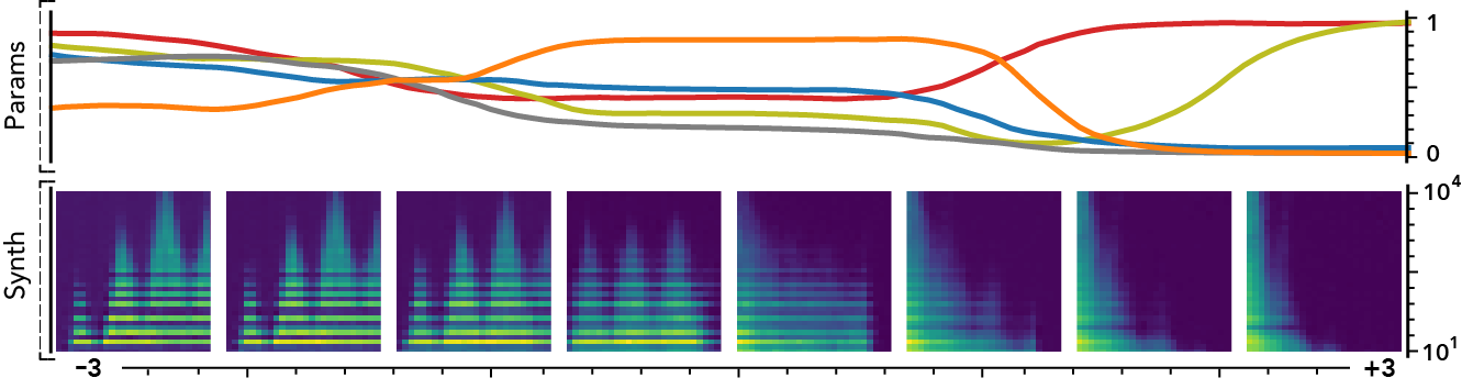
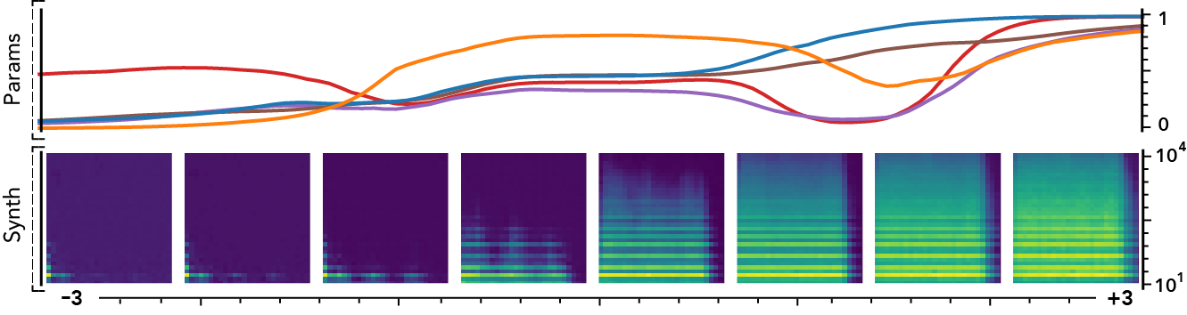
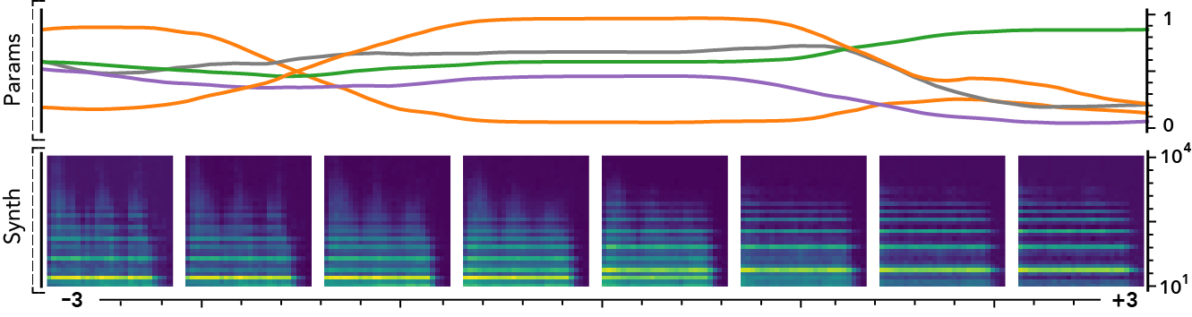
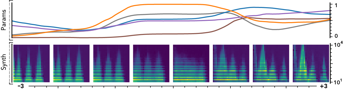
The latent dimensions can be seen as meta-parameters for the synthesizer that naturally arise from our framework. Moreover, as they act in the latent audio space, one could hope they impact audio features in a smoother way than native parameters.
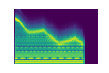
The following examples present the evolution of synth parameters and corresponding spectrogram while moving along a dimension of the latent space. Spectrograms generally show a smooth variation in audio features, while parameters move in a non-independent and less smooth fashion. This proves latent dimensions rather encode audio features than simply parameters values.
Audio space interpolation
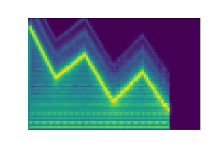
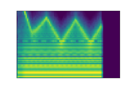
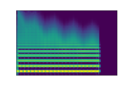
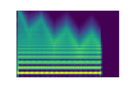
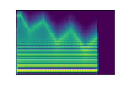
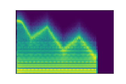
In this experiment, we select two audio samples, and embed them in the latent space as and . We then explore their neighborhoods, and continuously interpolate in between. At each latent point in the neighborhoods and interpolation, we are able to output the corresponding synthesizer parameters and thus to synthesize audio.
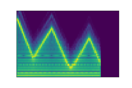
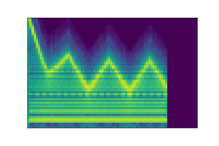
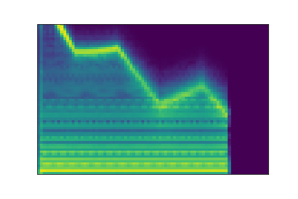
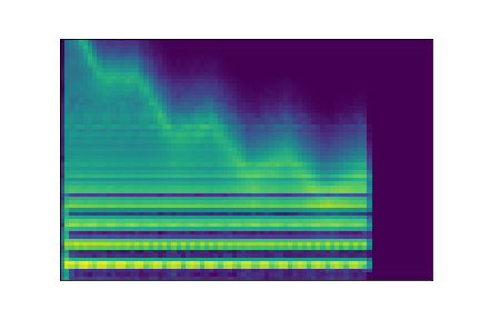
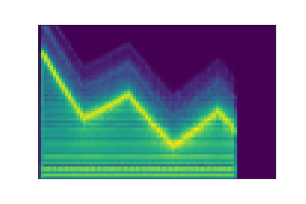
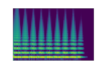
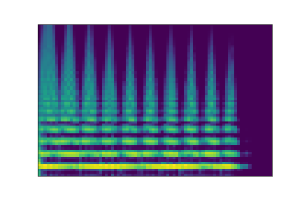
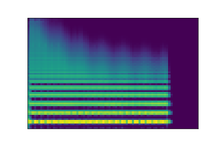
On the figure below, one can listen to the output and visualize the way spectograms and parameters evolve. It is encouraging to see how the spectrograms look alike in the neighborhoods of and , even though parameters may vary more.
| Audio | \(\mathbf{z}_0 + \mathcal{N}(0, 0.1)\) | Audio space | \(\mathbf{z}_1 + \mathcal{N}(0, 0.1)\) | Audio | ||
|---|---|---|---|---|---|---|
| Parameters | Spectrogram | Spectrogram | Parameters | |||
| PARAMS IMG | 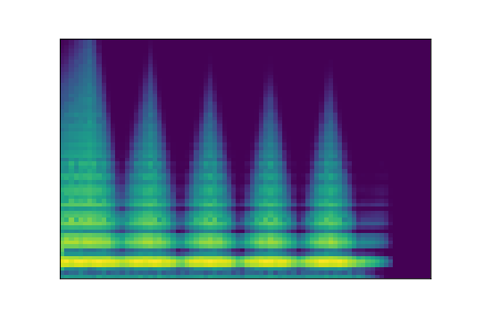 |
AUDIO SPACE IMG | 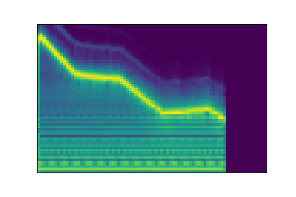 |
PARAMS IMG | ||
| PARAMS IMG | 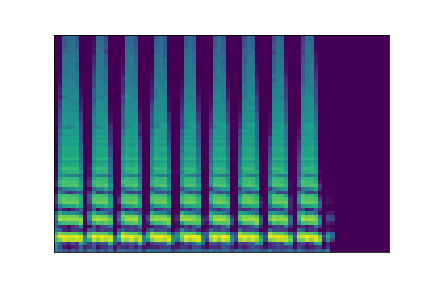 |
 |
PARAMS IMG | |||
| PARAMS IMG | 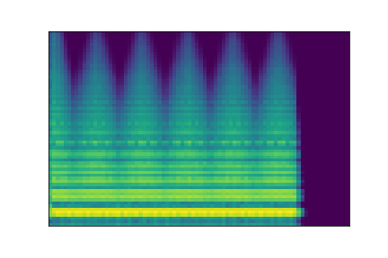 |
 |
PARAMS IMG | |||
| PARAMS IMG | 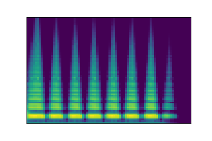 |
 |
PARAMS IMG | |||
| PARAMS IMG | 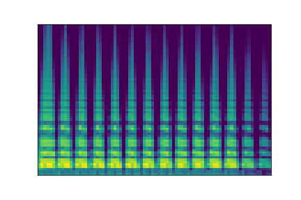 |
 |
PARAMS IMG | |||
| PARAMS IMG | 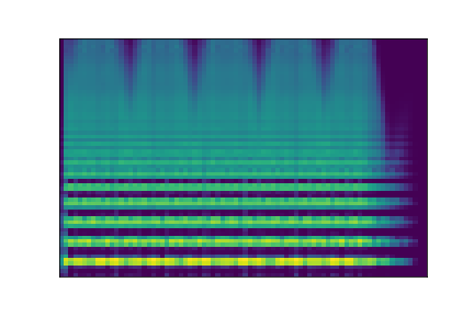 |
 |
PARAMS IMG | |||
| PARAMS IMG | 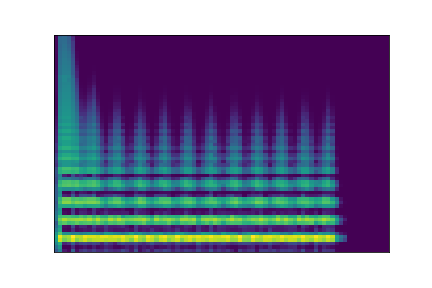 |
 |
PARAMS IMG | |||
| PARAMS IMG | 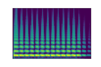 |
 |
PARAMS IMG | |||
 |
 |
 |
 |
 |
 |
 |
 |
Parameters inference
Here, we compare the accuracy of all models on parameters inference by computing the magnitude-normalized Mean Square Error () between predicted and original parameters values. We average these results across folds and report variance. We also evaluate the distance between the audio synthesized from inferred parameters and the original with the Spectral Convergence (SC) distance (magnitude-normalized Frobenius norm) and MSE. We provide evaluations for 16 and 32 parameters on the test set and an out-of-domain dataset in the following table.
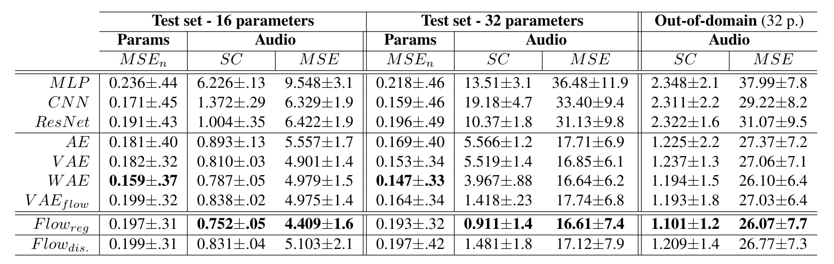
In low parameters settings, baseline models seem to perform an accurate approximation of parameters, with the providing the best inference. Based on this criterion solely, our formulation would appear to provide only a marginal improvement, with s even outperformed by baseline models and best results obtained by the . However, analysis of the corresponding audio accuracy tells an entirely different story. Indeed, AEs approaches strongly outperform baseline models in audio accuracy, with the best results obtained by our proposed (1-way ANOVA , ). These results show that, even though AE models do not provide an exact parameters approximation, they are able to account for the importance of these different parameters on the synthesized audio. This supports our original hypothesis that learning the latent space of synthesizer audio capabilities is a crucial component to understand its behavior. Finally, it appears that adding disentangling flows () slightly impairs the audio accuracy. However, the model still outperform most approaches, while providing the huge benefit of explicit semantic macro-controls.
Increasing parameters complexity. We evaluate the robustness of different models by increasing the number of parameters from 16 to 32. As we can see, the accuracy of baseline models is highly degraded, notably on audio reconstruction. Interestingly, the gap between parameter and audio accuracies is strongly increased. This seems logical as the relative importance of parameters in larger sets provoke stronger impacts on the resulting audio. Also, it should be noted that models now outperform baselines even on parameters accuracy. Although our proposal also suffers from larger sets of parameters, it appears as the most resilient and manages this higher complexity. While the gap between AE variants is more pronounced, the flows strongly outperform all methods (, ).
Out-of-domain generalization. We evaluate out-of-domain generalization with a set of audio samples produced by other synthesizers, orchestral instruments and voices, with the same audio evaluation. Here, the overall distribution of scores remains consistent with previous observations. However, it seems that the average error is quite high, indicating a potentially distant reconstruction of some examples. Upon closer listening, it seems that the models fail to reproduce natural sounds (voices, instruments) but perform well with sounds from other synthesizers. In both cases, our proposal accurately reproduces the temporal shape of target sounds, even if the timbre is somewhat distant.
Semantic dimensions evaluation
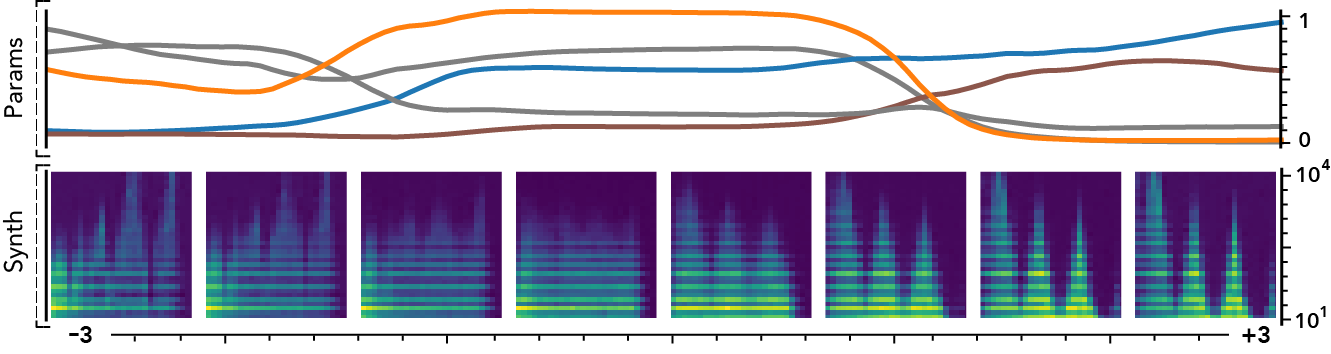
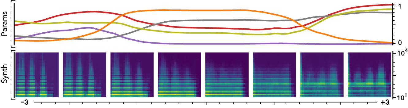
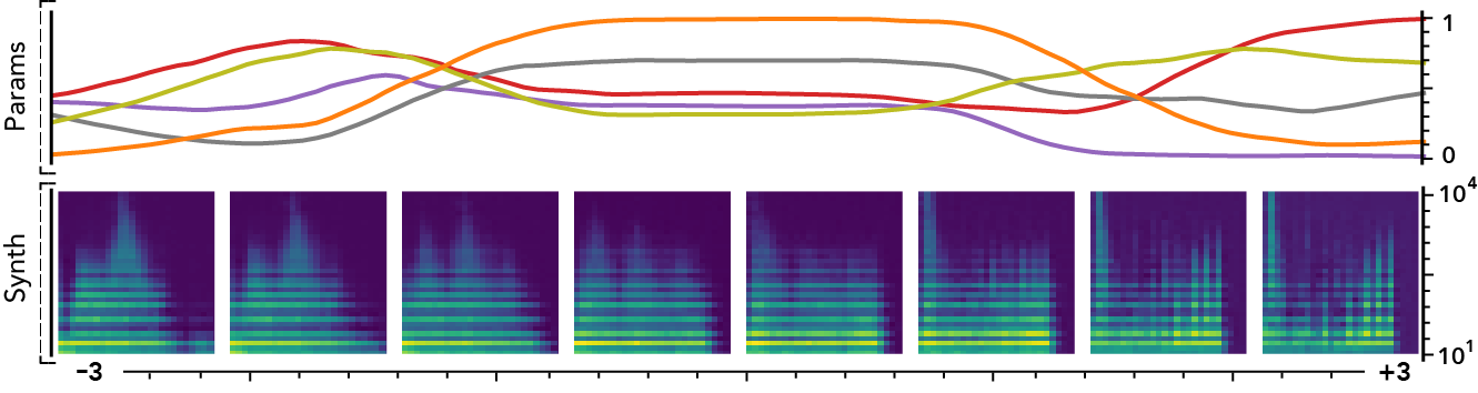
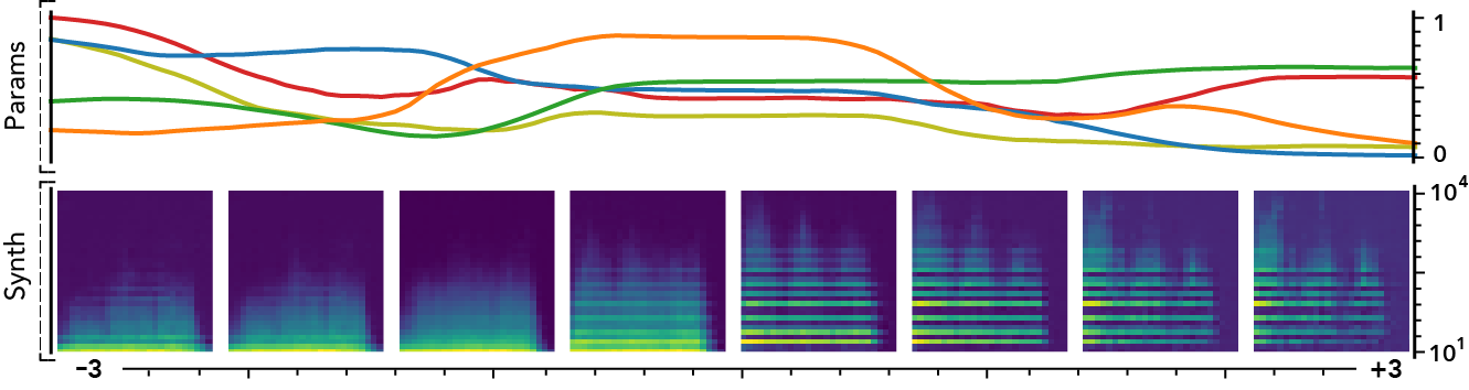
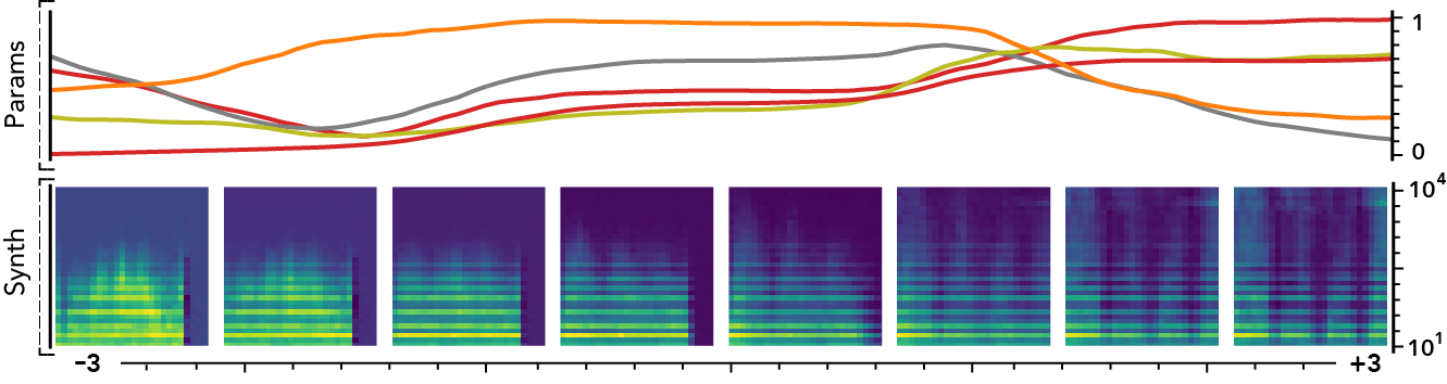
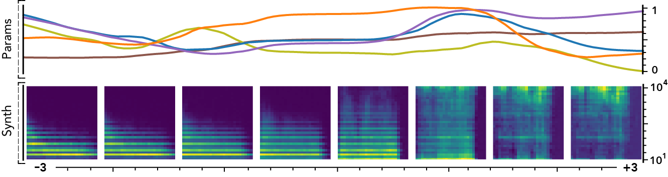
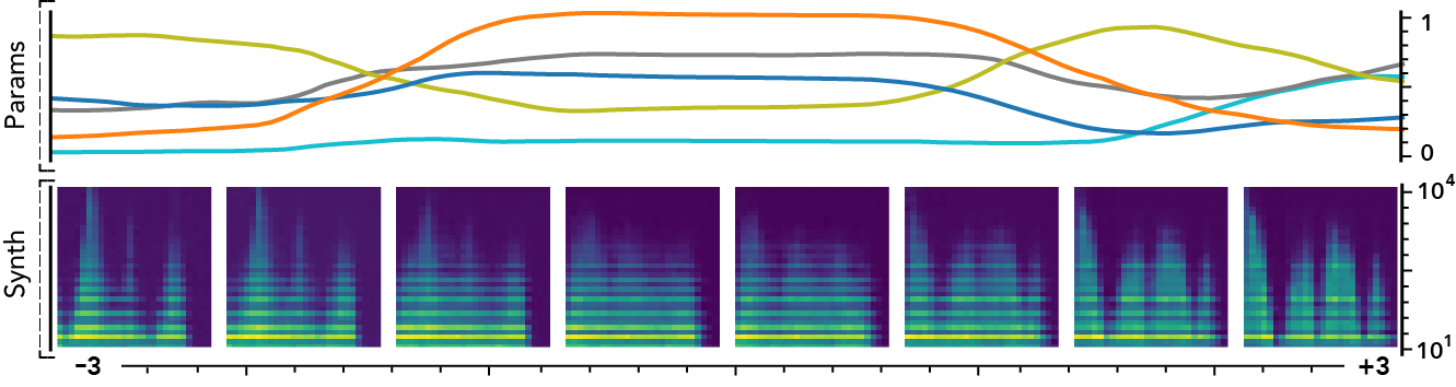
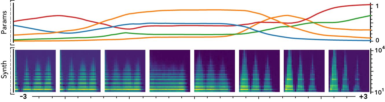
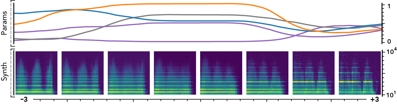
Our proposed disentangling flows can steer the organization of selected latent dimensions so that they provide a separation of given tags. As this audio space is mapped to parameters, this turns the selected dimensions into macro-parameters with a clearly defined semantic meaning. To evaluate this, we analyze the behavior of corresponding latent dimensions, as depicted in the following figure.
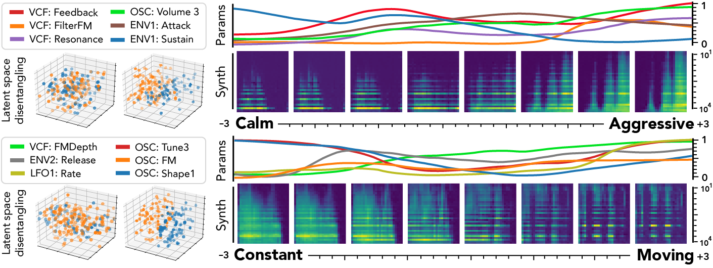
First, we can see the effect of disentangling flows on the latent space (left), which provide a separation of semantic pairs. We study the traversal of semantic dimensions while keeping all other fixed at and infer corresponding parameters. We display the 6 parameters with highest variance and the resulting synthesized audio. As we can see, the semantic latent dimensions provide a very smooth evolution in terms of both parameters and synthesized audio. Interestingly, while the parameters evolution is smooth, it exhibits non-linear relationships between different parameters. This correlates with the intuition that there are complex interplays in parameters of a synthesizer. Regarding the effect of different semantic dimensions, it appears that the [‘Constant’, ‘Moving’] pair provides a very intuitive result. Indeed, the synthesized sounds are mostly stationary in extreme negative values, but gradually incorporate clearly marked temporal modulations. Hence, our proposal appears successful to uncover semantic macro-parameters for a given synthesizer. However, the corresponding parameters are quite harder to interpret. The [‘Calm’, ‘Aggressive’] dimension also provides an intuitive control starting from a sparse sound and increasingly adding modulation, resonance and noise. However, we note that the notion of ‘Aggressive’ is highly subjective and requires finer analyses to be conclusive.
Vocal sketching
Finally, our models allow vocal sketching, by embedding a recorded vocal sample in the latent space and finding the matching parameters. Below are examples of how the models respond to several recorded samples.
Real-time implementation using Ableton Live
Not available yet.
Code
The full open-source code is currently available on the corresponding GitHub repository. Code has been developed with Python 3.7. It should work with other versions of Python 3, but has not been tested. Moreover, we rely on several third-party libraries that can be found in the README.
The code is mostly divided into two scripts train.py and evaluate.py. The first script train.py allows to train a model from scratch as described in the paper. The second script evaluate.py allows to generate the figures of the papers, and also all the supporting additional materials visible on this current page.
Models details
Baseline models.
In order to evaluate our proposal, we implemented several feed-forward deep models. In our context, it means that all the baseline models take the full spectrogram of one sample as input and try to infer the corresponding synthesis parameters . All these models are trained with a Mean-Squared Error (MSE) loss computed between the output of the model and the ground-truth parameters vector.
Multi-Layer Perceptron (MLP)
First, we implement a 5-layers MLP with 2048 hidden units per layer, Exponential Linear Unit (ELU) activation, batch normalization and dropout with . This model is applied on a flattened version of the spectrogram and the final layer is a sigmoid activation.
Convolutional Neural Network (CNN)
We implement a convolutional model composed of 5 layers with 128 channels of strided dilated 2-D convolutions with kernel size 7, stride 2 and an exponential dilation factor of (starting at ) with batch normalization and ELU activation. The convolutions are followed by a 3-layers MLP of 2048 hidden units with the same properties as the previous model.
Residual Networks (ResNet)
Finally, we implemented a Residual Network, with parameters settings identical to CNN. The normal path is defined as a convolution (similar to the previous model), Batch Normalization and ELU activation, while the residual paths are defined as a simple 1x1 convolution that maps to the size of the normal path. Both paths are then added.
Auto-encoding models
We implemented various AE architectures, which are slightly more complex in terms of training as it involves two training signals. First, the traditional AE training is performed by using a MSE reconstruction loss between the input spectrogram and reconstructed version . We use the previously described CNN setup for both encoders and decoders. However, we halve their number of parameters (by dividing the number of units and channels by 2) to perform a fair comparison by obtaining roughly the same capacity as the baselines.
All AEs map to latent spaces of dimensionality equal to the number of synthesis parameters (16 or 32). This also implies that the different normalizing flows will have a dimensionality equal to the numbers of parameters. We perform warmup by linearly increasing the latent regularization from 0 to 1 for 100 epochs.
For all AE architectures, a second network is used to try to infer the parameters based on the latent code obtained by encoding a specific spectrogram . For this part, we train all simple AE models with a 2-layers MLP of 1024 units to predict the parameters based on the latent space, with a MSE loss.
Families of auto-encoders (AE, VAE, WAE, VAEFlows)
First, we implement a simple deterministic AE without regularization. We implement the VAE by adding a KL regularization to the latent space and the WAE by replacing the KL by the MMD. Finally, we implement VAEFlow by adding a normalizing flow of 16 successive IAF transforms to the VAE posterior.
Our proposal
Finally, we evaluate regression flows () by adding them to , with an IAF of length 16 without using semantic tags. Finally, we add the disentangling flows () by introducing our objective defined in the paper.
Optimization
We train all models for 500 epochs with ADAM, initial rate 2e-4, Xavier initialization and a scheduler that halves the rate if validation loss stalls for 20 epochs. With this setup, the most complex model only takes $\sim$5 hours to train on a NVIDIA Titan Xp GPU.